A Counting Process Approach for Trend Assessment of Drought Condition


National Research Council, Institute for Bioeconomy, 50019 Sesto Fiorentino, Italy
*
Author to whom correspondence should be addressed.
Hydrology 2019, 6(4), 84; https://doi.org/10.3390/hydrology6040084
Submission received: 30 June 2019
/
Revised: 24 September 2019
/
Accepted: 25 September 2019
/
Published: 27 September 2019
Abstract
:This paper discusses some methodological aspects of the historical analysis of drought, particularly the trend assessment. The Standardized Evapotranspiration Index (SPEI) is widely used as a measure of drought condition. Since different SPEI thresholds allow classifying the risk into moderate, severe, and extreme, the drought occurrence becomes a counting process. In this framework, would a statistical trend test based on a Non-Homogeneous Poisson Process (NHPP) give a similar result of the nonparametric Mann–Kendall (M-K) test? In this paper, we demonstrate that the NHPP approach is able to characterize the information given by the classical M-K approach in term of drought risk classes. Furthermore, we show how it can be used to reinforce the framework of drought trend analysis in combination with a standard non-parametric approach. At a global scale, we find that: (1) areas under increasing risk of drought identified by the NHPP approach are considerably larger in comparison to those identified by M-K; and (2) the results of the two tests are different during crucial periods such as hydrological droughts in winter and spring.
1. Introduction
As a consequence of the increasing interest in the change of natural resources available due to climate change, many studies properly invest their efforts to address the management of such resources. Among others, water management plays a key role since water scarcity will be one of the main issues to be addressed by human beings [1,2], especially because of its subsequent effects on, the agricultural sector. Thus, many studies consider it of prominent importance to detect changes in temporal trends of drought, particularly at the regional scale. Drought is the result of a complex interaction among precipitation deficiencies, excessive evapotranspiration and the demands of water use. Whereas aridity is permanent and occurs only in low rainfall–high evapotranspiration areas, drought is a temporary feature that occurs mostly in all climatic zones. The definition of drought varies according to five types: meteorological, hydrological, agricultural, socioeconomic, or groundwater. This depends on the duration of the reduction in the amount of precipitation and the contributing variables that affect evapotranspiration, such as temperature, humidity, and wind. A complete review of drought definitions and concepts is given in [3].
In fact, the Earth warming intensifies the global hydrological cycle by increasing the globally averaged precipitation, evaporation, and runoff. In this framework, the Standardized Precipitation Evapotranspiration Index (SPEI) [4] is widely used since it combines the sensitivity of the Palmer Drought Severity Index (PDSI) [5] to the changes in evapotranspiration with the multi-temporal feature of the Standardized Precipitation Index (SPI) [6]. The possibility of being scale-free, i.e., calculated for a variety of time scales, allows SPEI to monitor both short-term water supplies and long-term water resources and, consequently, to be proper for either agricultural or hydrological drought. Recall that agricultural drought is mostly linked to soil moisture conditions that respond to precipitation anomalies on a relatively short scale, whereas hydrological drought regards groundwater, stream-flow, and reservoir storage that reflect the long-term precipitation anomalies.
Within this context, the trend analysis is an important tile to start the risk management associated with these type of events and the choice of the statistical methods to assess trend is one of the causes that determine differences in the results of studies devoted to this subject [7,8,9].
In general, the trend analysis of a variable includes both the assessment of direction and magnitude. Trend direction reveals whether there is an increasing (positive) or decreasing (negative) dependence of the variable on-time, while trend magnitude expresses the measure of this variation in terms of relative change per unit of time. The Mann–Kendall (M-K) statistical test has been frequently used to assess the significance of trends in hydro-meteorological time series because it requires fewer assumptions than the parametric tests [10]. Many studies apply M-K test to assess the SPEI trend either locally or globally. For instance, Vicente-Serrano et al. [11] used M-K test to assess trends in the seasonal SPI and SPEI time series representative of different regions obtained through principal component analysis in Bolivia; Li et al. [12] combined M-K trend test of SPEI time series and an analysis of the average variation of dry episodes duration in a region of South Tibet; Liu et al. [13] used the analysis of SPEI trend for classifying the risk of the crop yield; and Tan et al. [14] used M-K test for Malaysia drought trend assessment where droughts are identified by means of SPI. About SPI, which is straightforward comparable to SPEI being built in a very similar methodological framework, several studies have used a parametric approach to evaluate the change in time of droughts. Among others, Moreira et al. [7] applied a log-linear model to assess significant change in the fixed classes of risk; Krysanova et al. [15] applied both linear and general linear models to account for drought change in the Elba basin; and Bazrafshan [16] proposed a trend drought assessment of Iran based on both the nonparametric and parametric test using either SPI or SPEI.
Another approach for the analysis of drought trend is to investigate the statistical properties of drought. In particular, once SPEI has been fixed as drought measure, it is possible to calculate the duration, severity, and intensity of droughts throughout the time series [17]. This computation relies on the assumption that a drought event is considered to occur at a time when the value of SPEI is continuously negative and ends when SPEI becomes positive. Then, the return period of duration, severity, and intensity properties gives a tendency of drought expectation for the future. For instance, Mishra and Singh [18] used the annual values of drought severity for frequency analysis and fit a distribution to analyze the associated risk of droughts using the exceedances’ probability, while Mortuza et al. [19] used a copula approach to identify the joint probability distribution of drought duration and severity, then computed the return period of drought according to different thresholds. Finally, Onyutha [20] introduced a modified version of the extreme value distribution used for frequency analysis of drought extreme events, which takes into account the non-stationarity of the data.
The scientific question posed in this paper regards how to evaluate the trend of SPEI in a specific drought risk class among moderate, severe and extreme. The typical methodological framework for trend analysis in hydrology is to combine M-K for significance and -Sen method for direction and magnitude. The M-K is a powerful tool that can also be extended to the detection of a trend in non-normally distributed time series. For instance, Yue et al. [21] examined the power of the M-K test, i.e., the probability of rejecting a null hypothesis when it is false for a few commonly used distributions in hydrology: the extreme value distributions, the Pearson type 3, and the lognormal. Even though the advantages of such a nonparametric test, for example, the assumption of normality or of variance homogeneity are not needed, there are several shortcomings that can influence the result of the M-K and need to be addressed: (i) the serial correlation in the time series [10,22,23]; and (ii) the dependence of test power on the magnitude of trend, sample size, and the amount of variation within a time series [21].
Here, we propose a trend test for the different classes of drought risk based on the Poisson process and we compare its results with those of the M-K test. In fact, when a truncation level is imposed, the exceedances of a climatological time series can be modeled as a point process. In the framework of the time series of SPEI values calculated at a specific time scale and for a given month, we can consider the inter-arrival times—years in this case—between drought episodes as independent and identically distributed. Consequently, the point process becomes a counting process (among many, see Par. 4.2 of [24]) and the natural distribution used to describe such a counting process is the Poisson distribution. The latter is entirely characterized by a unique parameter: the intensity or rate of the process, which can be interpreted as the mean number of drought episodes per unit of time (years). Furthermore, if the arrival rate does not remain constant through time, then it follows a Non-Homogeneous Poisson Process (NHPP). This framework is particularly useful because, as demonstrated by Park et al. [25]: “drought expressions by a statistical index such as SPI can be distorted by stationary assumption and cautious approach is needed when deciding drought level considering climate changes”. We consider the use of a special case of the NHPP: the power law process defined in [26]. The power-law functional form used to model the dependence of the process intensity on time suggests the use of the test for time-trend analysis. This approach is commonly used in risk evaluation, for example Ho [27] used it to evaluate volcanic eruptions time-trend or in lifetime analysis. Nevertheless, applications for SPI in this theoretical framework already exist, for example Achcar et al. [28] used NHPP to identify change points in time series of droughts in Brazil. The main advantage of this approach is that the trend is completely determined by the exponent of the power-law [27].
Moreover, we present the computer code used for the computation of SPEI time series at a global scale as well as that for the trend analysis. The part of code regarding the SPEI computation starts from that proposed by Beguería et al. [29] and it is based similarly on the precipitation and evapotranspiration time series of the CRU dataset [30]. Our code [31] is openly accessible from the link https://zenodo.org/badge/latestdoi/194230602, and differs from that released by Beguería [32]: (1) because it is based on the raster [33] instead of ncdf4 R package; and (2) because it is possible to set the time window for the reference period to be used in the parameter estimation phase. The SPEI dataset resulting from our computation is comparable in principle with the SPEI global database released by Beguería et al. [29]; however, the comparison is not feasible since the code released by these authors does not allow setting the reference period and, moreover, it seems to contain a bug in the part regarding the expansion of potential evapotranspiration from the mm/day scale to mm/month.
This paper is organized as follows.Section 2 contains a brief description both of the dataset and the programming code used to calculate the SPEI; in particular, Section 2.3 introduces our methodological proposal for testing the significance of SPEI trend and its nonparametric counterpart, the Mann–Kendall test; and Section 3 presents a comparison of the two methods in terms of differences for 3, 6, 12, and 24 monthly temporal scales either in the form of global maps or box plots. Finally, Section 4 concludes the paper with some discussion. In this study, we used R software [34], and SPEI [35] and modifiedmk [36] R packages for SPEI calculation and M-K test computation, respectively.
2. Materials and Methods
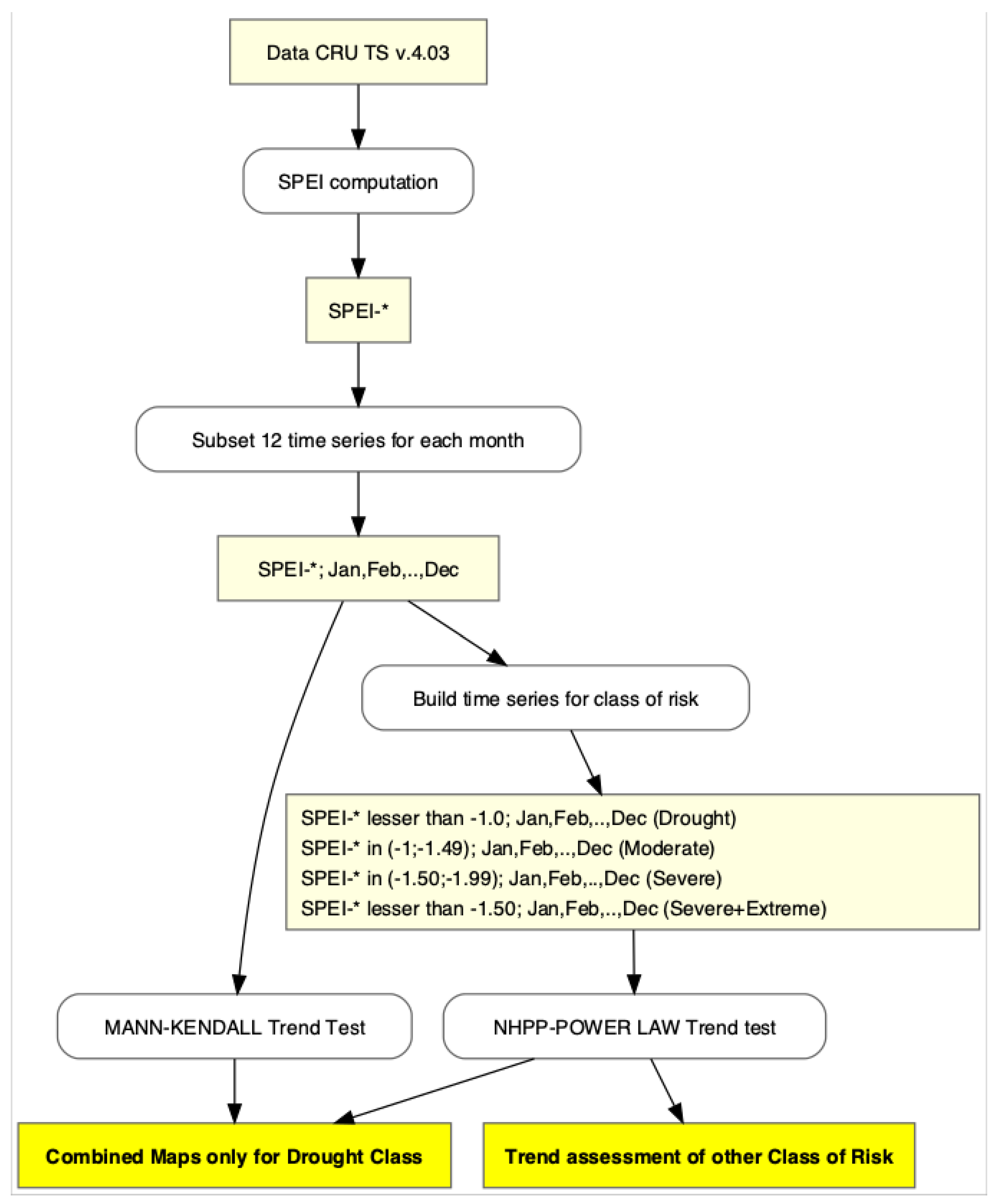
In this section, we briefly describe the dataset, the approach for the SPEI computation, and the two methods used for trend analysis. To facilitate the understanding of the reader, we anticipate the content of the following paragraphs in the technical flow chart of Figure 1. The computer code used for the analysis done in this paper is fully downloadable. More details on how to use the code to reproduce the results obtained in this work are given in Appendix A.
2.1. Data
We used the CRU TS v.4.03 gridded time-series dataset, released by Climatic Research Unit, University of East Anglia [30]. The dataset covers all land areas (excluding Antarctica) at 0.5° horizontal resolution and the period 1901–2018. As declared by the authors, several areas at the global level present drawbacks in the monthly time series, depending on the number of stations which contribute to the gridding of monthly anomalies. Because of this limitation, following the International Research Institute for Climate and Society (IRI) method, we applied a dry mask with a 3 mm monthly threshold that guarantees from errors in the SPEI computation. More specifically, we set to missing the whole values of those time series which yearly average precipitation is less than 73 mm (0.2 mm per day multiplied by 365 days). As a result, we obtained a dry mask for the desert zones of the globe, the widest being in the Sahara desert.
2.2. Data Preparation for Trend Analysis
The phase of data preparation for trend analysis is composed of two parts: (1) the computation of SPEI time series from precipitation and evapotranspiration data at 3-, 6-, 12- and 24-month scale of aggregation; and (2) the subsetting of SPEI time series for each month of the year. The final output of this phase is represented by 48 time series resulting from the 4 aggregation scales (3-, 6-, 12- and 24-month) multiplied by the 12 months of the year. Thus, for each month, we have a time series of 118 values corresponding to the number of years in the time window 1901–2018. Let us label the SPEI time series as SPEI-3, SPEI-6, SPEI-12, and SPEI-24 according to the scale of aggregation such that, for example, the time series of SPEI at 6-month for March is briefly indicated as SPEI-6 March. The latter is composed of the values of SPEI calculated for the 118 months of March from 1901 to 2018. Recall that the SPEI time scale for a specific month refers to the time window from which the amount of data used for the calculation is extracted, i.e., in the case of this work, the cumulated precipitation and evapotranspiration for the last 3, 6, 12 and 24 months. Back to the example of SPEI-6 March, this means that each yearly value of the time series is calculated based on the data from October to March. At a global spatial scale, this calculation is repeated 259,200 times, which corresponds to the number of grid cells of the CRU dataset at 0.5° spatial resolution.
To obtain this set of time series, we followed the SPEI original definitions proposed by Vicente-Serrano et al. [4], who fitted the long-term precipitation minus potential evapotranspiration time series to a log-logistic distribution, in order to transform the data into a standard normal variable with zero mean and variance equal to one. More specifically, the parameter fitting of the log-logistic distribution is done in the 50-year time window 1951–2010 by means of unbiased probability weighted moments, then used to find the cumulative distribution of the observed precipitation minus potential evapotranspiration. Finally, by back-transforming, the probability value on the standard Gaussian distribution gives the desired SPEI value. Thus, the SPEI has a Gaussian configuration in which the mean is zero and its value corresponds to units of standard deviation from the long-term mean of the standardized distribution. Consequently, the magnitude of the deviation from the mean is a probabilistic measure of the severity of a wet or dry event. Since this study focused on droughts, in Table 1, we report only the thresholds that identify the severity of a dry event.
At the end of this subsection, it is worth hinting at the debate that regards the type of distribution to be used for the transformation of data into probabilities. Stagge et al. [37] demonstrated that the Generalized Extreme Value (GEV) distribution is better than the log-logistic originally proposed by the authors of SPEI [4] for the observations fitting. However, Vicente-Serrano et al. [4] replied by highlighting that the results obtained by Stagge et al. [37] strictly depend on the data used and the power of test used by them is not strong enough to refute the original choice of the log-logistic distribution [38].
2.3. Statistical Tests for Trend Analysis
To investigate the statistical significance of the two trend tests presented in this paper, we started from the SPEI time series at the various scales, as described in Section 2.2. Then, we extended the classification in Table 1 by aggregating the moderately, severely, and extremely dry classes into a unique class that we label as Drought, and similarly the severely and extremely dry classes into the Severe+Extreme one. At the same time, we excluded the Extreme class because we find that the dataset is not consistent with the Poisson configuration (see Section 2.3.2 for details). The final list of drought classes analyzed in this study is reported in Table 2.
The aggregation into a wider class that includes the whole dry events identified by SPEI less than −1, i.e., the Drought class, is particularly useful for the scope of this study. In fact, while the M-K test operates by using all the data throughout the time series and, consequently, it could possibly give a significant trend of increasing dry events whenever there is an increasing number of events which SPEI value is less than 0, the test based on NHPP approach is able to model only the negative exceedances of a specific threshold among those reported in Table 2. Note that it would also be possible to apply the M-K by fitting the data to other known distributions tailored for the analysis of extreme events, however in this case we are required to estimate the parameters of such distributions. A comparison of the two approaches is only possible by taking the drought episodes identified by SPEI value less than 0 in the case of M-K and the defined Drought class, i.e., SPEI value less than −1 in the case of NHPP trend test. This assumption is plausible if we consider the drought in term of its associated risk; in other words, we assume that the events identified by the thresholds 0 and −1 have, on average, the same severity. For the sake of clarity, we use the plot in Figure 2 to exemplify the methodological differences of the M-K and NHPP approaches.
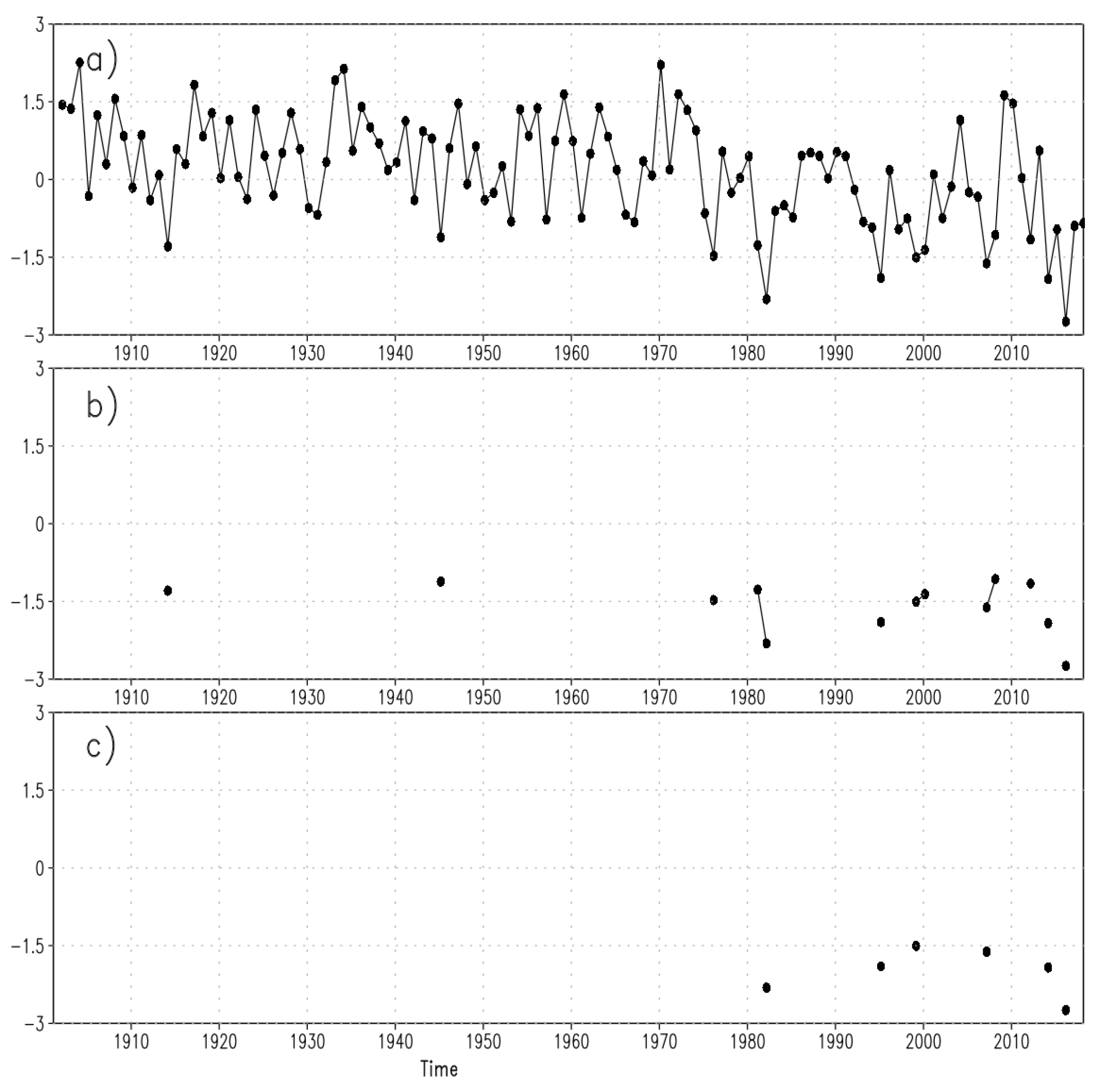
Figure 2 reports the SPEI-6 March values from 1901 to 2018 at location 37° N, 2.25° W of Iberian peninsula and it is divided into three panels: (a) the complete time series, i.e., the SPEI-6 values of March for each year; (b) only the values exceeding the negative threshold of −1, i.e., those events belonging to the Drought class; and (c) only the values less than −1.5, i.e., the events in the Extreme+Severe class. Now, the M-K test works with the time series visualized in Figure 2a and the correspondent test statistic is built based on the sequences of + and − that are generated from this time series being its values positive or negative, respectively. The reader is referred to the seminal paper of Mann [39] and to the book of Kendall [40] for further details. Finally, once the levels of I Type Error (to refuse a true hypothesis) has been fixed, then the test results in accepting or refusing the null hypothesis that states the absence of a trend in the data. The direction of the trend, if any, can be identified by other nonparametric methods, for instance, the Sen’s slope [41]. On the contrary, the NHPP test is applied over the events exceeding the thresholds indicated in Figure 2b,c, and its statistic is based on the modeling of the probability of arrival of those events. From the example in Figure 2, it appears quite clear that the frequency of the drought episodes is increased in the last part of the observation period. However, while the increase is evident for the NHPP approach because it takes into account only the exceedances (Figure 2b,c), the M-K test has to deal with the high variability of the entire time series values (Figure 2a)). Indeed, in this example, the NHPP gives a positive trend while the M-K results in a no trend.
Another issue that has to be taken into consideration is the statistical power of the test. For instance, Yue et al. [21] showed in their paper on the use of non parametric tests for trend detection in annual maximum daily streamflow data of 20 basins in Canada that the power of M-K test depends on “the magnitude of trend, sample size, and the amount of variation within a time series”. They found that the power of the M-K test proportionally increases as the magnitude of the trend as well as the sample size increase, while it decreases “as the amount of variation increases within a time series”.
Methodological details of both the trend test based on M-K and NHPP are given in Section 2.3.1 and Section 2.3.2, respectively.
2.3.1. Mann–Kendall Trend Test
Most of the work on nonparametric tests was originally done by assuming that there is an underlying continuous distribution, such that the building of the test statistic can be done on the basis of known distributions. In some cases, the statistic works out to be approximately normal, which makes the parameter estimation easier. However, it may happen to have ties when data are rounded or the variable is naturally discrete. In other words, a tied group is a set of sample data having the same value. In these cases, the standard assumptions do not hold. One simple way to deal with ties is to use randomization tests such as permutation tests or bootstrapping. Another issue is the influence of autocorrelation on the results of trend detection. This fact suggests following some methodological approach to assess the significance of the trend in serially correlated time series. For instance, von Storch and Navarra [23] proposed the pre-whitening approach that is based on the removal of the lag-one AR1 autoregressive component, while Hamed and Ramachandra Rao [42] introduced a theoretical framework to calculate the variance of the Mann–Kendall test for autocorrelated data, which is an empirical formula to compute effective sample size (ESS). Yue et al. [22] argued that “pre-whitening a positive AR(1) will also remove a portion of the trend; hence, the slope of the trend after pre-whitening is smaller than the slope before pre-whitening. This will lead to an underestimation of a significant trend”. Nevertheless, Zhang and Zwiers [43] replied to indicate how to correctly apply a pre-whitening approach when a serial correlation is identified in the data. Another approach was proposed by Burn and Hag Elnur [10], which uses a permutation test to account for the correlation structure in the data. A more trivial modified version of the M-K test to account for serial correlation is the Mann–Kendall–Sneyers test [44]. In this work, the non-parametric Mann–Kendall (M-K) test was used to detect trends in time series of SPEI values at a time scale of 3, 6, 12, and 24 months. Following a common methodological scheme (see, for example, [12,16,45]), we applied the pre-whitening procedure proposed by von Storch and Navarra [23] to eliminate the effect of time series serial correlation on the result of trend analysis. The interested reader may refer to the work of von Storch and Navarra [23] for technical details. In particular, we applied the pre-whitening method only to the data series at 24-month time scale because, for construction, they contain exactly the same precipitation and evapotranspiration data for 12 out of 24 months. For example, the SPEI-24 of November 1950 is calculated by using the data from December 1948 to November 1950, and the SPEI-24 of November 1951 is calculated by using the data from December 1949 to November 1951. This means that for the calculation of SPEI-24 of November 1951 the same set of data from December 1949 to November 1951 is used. Notice that this is not an issue for the SPEI-3, SPEI-6, and SPEI-12, for which time series values can be considered as independent.
Then, we used the Sen’s slope method [41] to evaluate the direction of the trend. A negative slope value indicates the increasing of drought events, whereas a positive slope the decreasing of such events. For the analysis described in this section, we used the modifiedmk R package for the computation of both M-K test significance and the trend Sen’s slope [36].
2.3.2. Non-Homogeneous Poisson Process (NHPP) with Power Law Trend Test
Let be the cumulative number of drought episodes in a given class of risk and at a given SPEI time scale that are observed at times during the interval . Since the drought episodes occur independently at some random time in , is non-decreasing, right continuous, and increases with unit jumps. On these theoretical basis, is a point process with values in . Let us define the sequence of inter-arrivals at instant jumps as for . Then, is the counting process of the number of years that pass between drought episodes. Furthermore, let us assume that the realizations of drought episodes follow a Poisson law, i.e.,
Then, is a Poisson process with intensity or rate , which can be interpreted as a mean number of jumps per unit of time. Recall that and . The Poisson distribution is unimodal and skewed to the right over the values. Its mean is equivalent to its variance. When is assumed to be not constant throughout the period of observation, the process is named a Non-Homogeneous Poisson Process (NHPP). In this framework, we need to allow to be a function of time, , in order to verify if the drought episodes below a given threshold are generated from a non-stationary process. This NHPP has mean function , where is the vector of unknown parameters and intensity function:
Then, we fully characterize the process by specifying the functional form of according to a power law as given in [26]. Consequently, the mean and intensity functions become, respectively:
and
where .
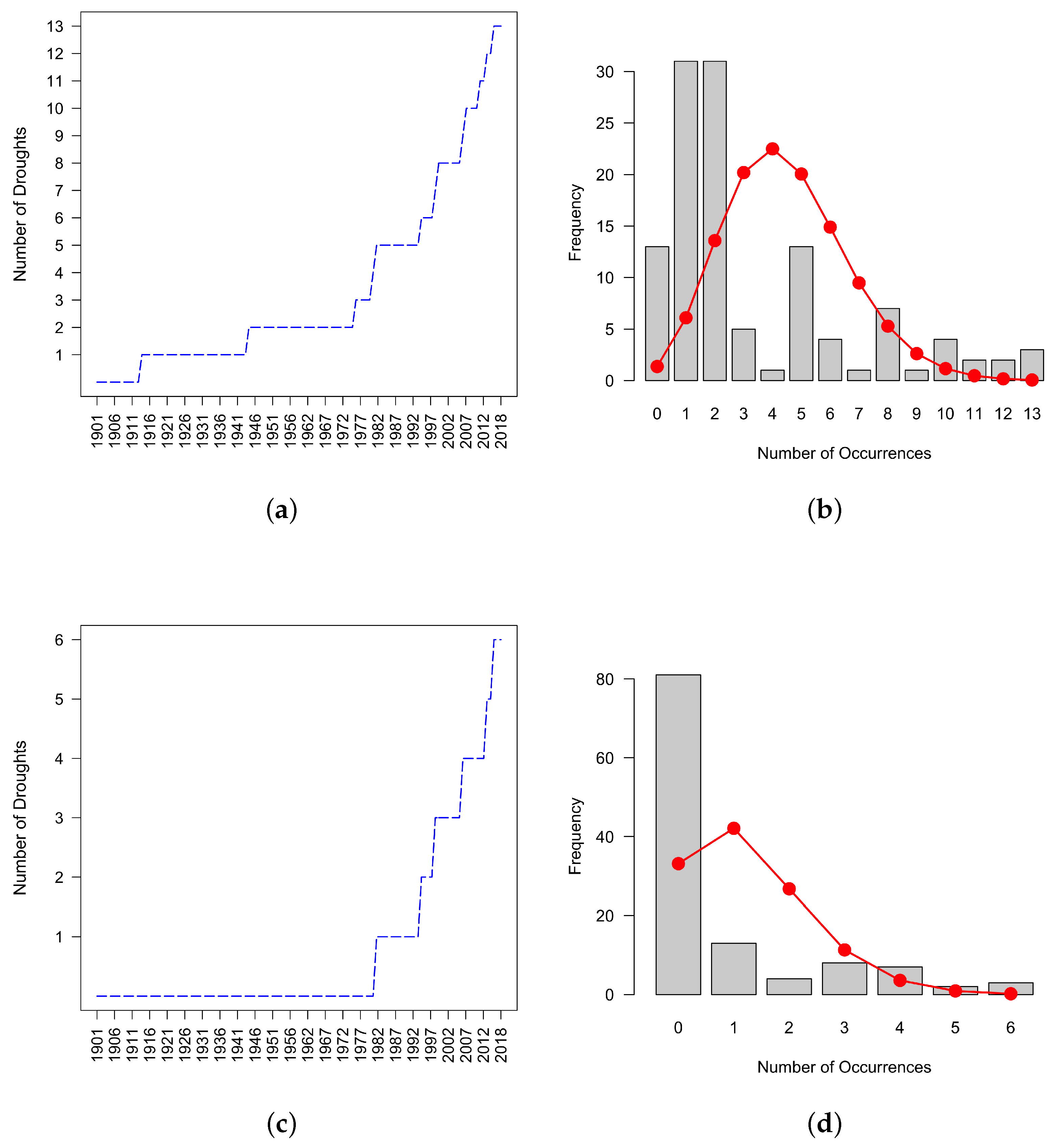
Let us again use the example in Figure 2 to illustrate the NHPP theoretical framework. In Figure 2b,c we take the instant times at which the drought episodes occur and use them to draw the cumulated function of drought episodes. The result of this action is plotted in Figure 3a,c, where the x-axis represents the sequence of years from 1901 to 2018 for the month of March and the y-axis is the number of drought episodes occurred in the class Drought and Severe+Extreme, respectively. By visualizing the histograms in the correspondent Figure 3b,d, it appears evident the concept of counting process: for each time ordered drought episode in the x-axis, the y-axis reports the number of years to wait for the successive episode. The red line represents the fitting of the data to the Poisson distribution. In the case of this example, the test gives a good fit as a result; nevertheless, it appears from the graphs that there exists a strong dependence of the process intensity on time. That is why we use NHPP.
We applied a goodness-of-fit test to verify if the proposed Poisson distribution is consistent with our dataset. This test is based on the likelihood ratio test using the Maximum Likelihood method to estimate the parameters. We used the goodfit function in the vcd R package [46], which also gave the plots reported in Figure 3. The result obtained by this test convinced us to exclude the Extreme class from the analysis. However, the proposed approach holds for the other classes, namely Drought, Moderate, Severe, and particularly for the Severe+Extreme, which allowed us to analyze the excluded drought episodes. The goodness-of-fit test shows a good approximation to the Poisson distribution at a global scale for all of them (not shown). It is worth reporting that the goodness-of-fit test for the Extreme class holds in wide areas of the globe, which suggests considering its inclusion in the context of local-scale analysis.
The good approximation of data to the Poisson distribution allows us to adopt the methodological scheme described above. Thus, we can model droughts by means of NHPP where a power law is used to model the dependence of the on time and, supposing that violations from a predetermined threshold are observed in at time , we can define the test statistic as follows:
Then, we obtain the maximum likelihood estimators of both the two power law parameters and [26], and the intensity of the process becomes [47]:
In this framework, the analysis of droughts time-trend is completely determined by : for , the intensity of droughts is increasing; it is decreasing for ; and it is constant for . In the latter case, the process corresponds to a homogeneous Poisson. Under the null hypothesis , the statistic has a distribution and, fixing as the acceptance level of I Type error, the test results in rejecting the null hypothesis if
where is the -percentile of the distribution with degrees of freedom.
The main advantage of the power law characterization is that the trend is completely determined by replacing with [27].
3. Results
This section presents box plots and summary tables of the M-K and NHPP test results at the level of significance. Illustrative maps showing the different spatial configuration of drought risk tendency between the two methods are also presented.
3.1. Differences between the Two Methods
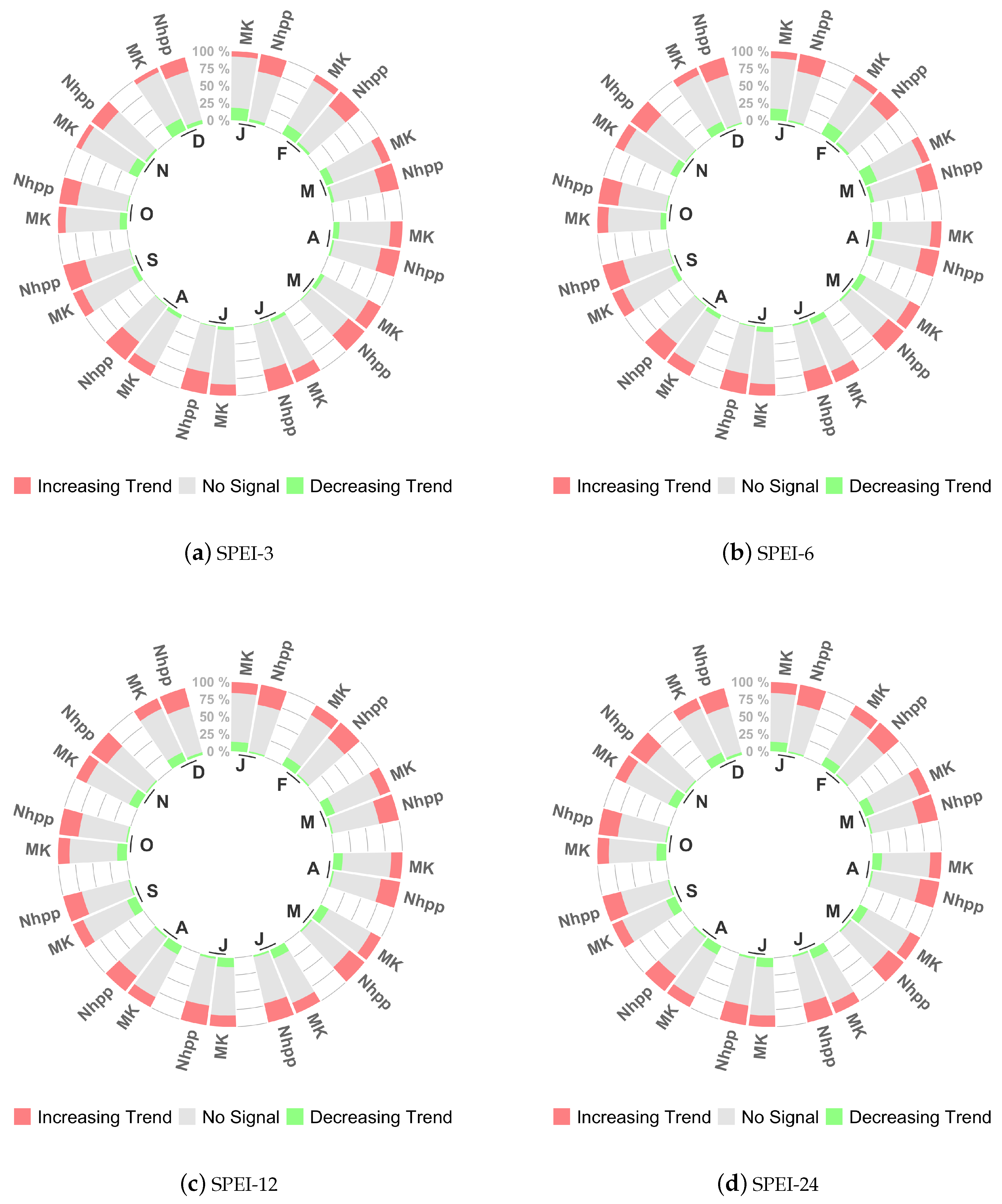
As mentioned in Section 2.3, to compare the two methods, we focused the analysis on the defined Drought class, since it includes all the possible dry events identified by SPEI (see Table 2). The result of this comparison is summarized by the number of grid cells out of the total 259,200 where the two tests give a significant trend. Figure 4 reports the relative number of grid cells where the test gives positive trend (red), i.e., the increasing on time of the drought events, negative trend (green), and non-significant trend (light grey), for each month of the year and for each index time scale.
It appears that the cases of a positive trend identified by the NHPP test are more numerous than those found by M-K. This result is more accentuated in the case of SPEI-24, suggesting a sharp difference of the increasing risk evaluation between the two methods for hydrological droughts at a global level. Besides, for the months from October to April of the shorter scales SPEI-3 and SPEI-6, a significant number of cases with the negative trend by the M-K to NHPP also emerges. Table 3 reports in details the percentage of variation of the cases with positive trend given by NHPP test to M-K.
These results are strictly locally dependent. This fact suggests investigating their spatial distribution. The maps in Figure 5 and Figure 6 show the difference results at a spatial scale for SPEI-6 March. These illustrative maps serve only to explain how the methods differ from one another rather than to summarize the findings at a global scale. Nevertheless, the interested reader could generate the maps for a specific month and time scale by using the computer code described in Appendix A.
Recall that, for M-K approach, a negative slope value indicates the increasing of drought events, whereas a positive slope the decreasing of such events. On the contrary, for the test based on NHPP, the increasing of drought events corresponds to a value of (see Section 2.3.2). However, for the sake of simplicity, we adopt the same coding for both the test approaches, that is
- 1 for positive trend, i.e., the increasing of drought episodes
- 0 for non-significant trend
- for negative trend, i.e., the decreasing of drought episodes
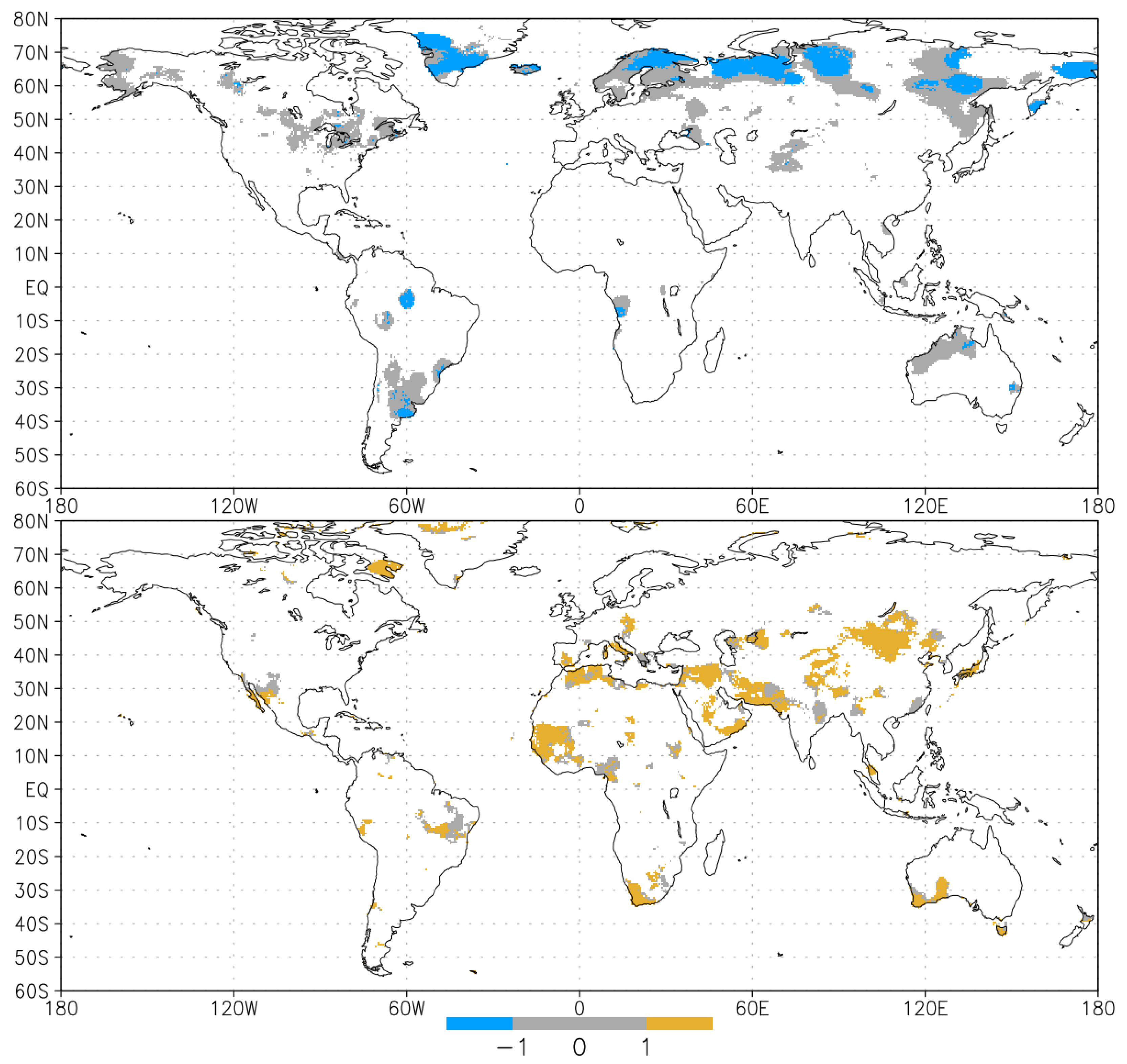
The map in Figure 5 shows the cases where the M-K gives a negative (top) and positive trend (bottom) and how the NHPP test responds in the same areas.
For the case of SPEI-6 March, it emerges that a large portion of the negative trend cases (blue + grey in Figure 5, top) given by M-K are changed to non-significant trend (grey in Figure 5, top), whereas the complementary situation, i.e., the positive trend cases (yellow+grey in Figure 5, bottom) changed to non-significant trend (grey in Figure 5, bottom) is less evident and applies only locally. These results are similar to the findings described in Section 3.1, in particular with the greater number of negative trend cases identified by M-K compared to NHPP for the months from October to April. On the other hand, the map depicted in Figure 6 confirms that the number of positive trend cases identified by M-K is significantly smaller than that found by the NHPP approach.
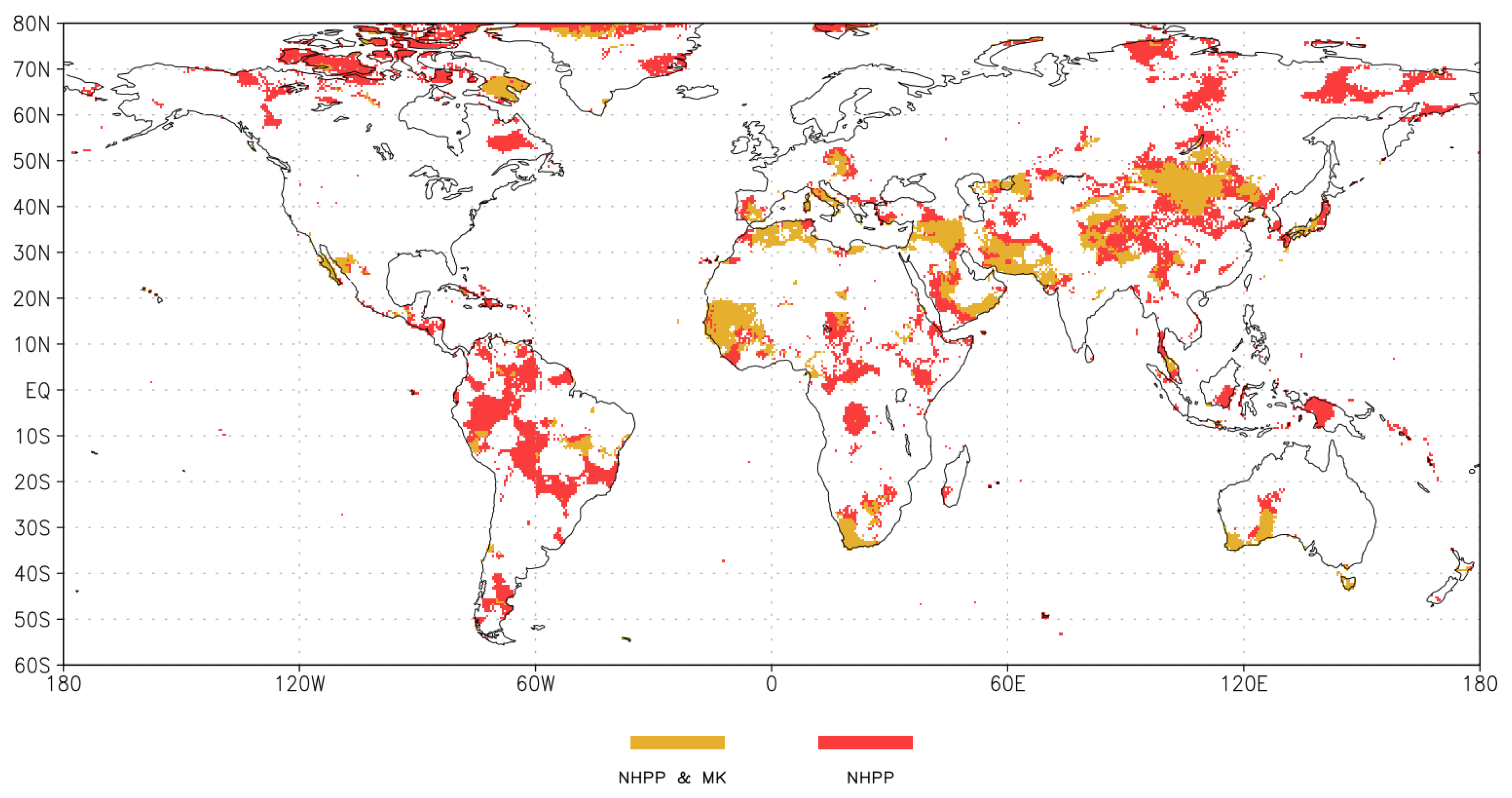
In fact, the map in Figure 6 reports only the cases of a positive trend for SPEI-6 March resulting from both the tests presented in this study. From this map, it clearly appears how the areas under risk of increasing drought events are significantly larger if the NHPP approach is used instead of M-K to test the trend. Notice that, in this map, the response of positive trend given by NHPP is represented by the union of yellow and red areas.
3.2. Characterizing Trend Results by Drought Risk Class
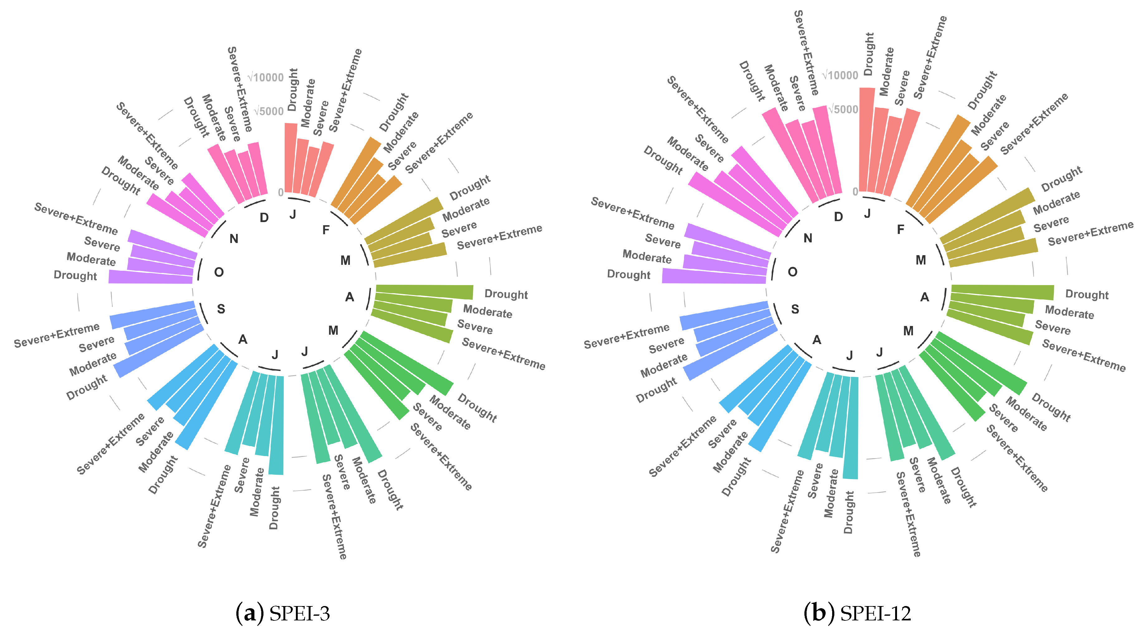
An advantage of using a counting process approach for testing the trend, in the case of those drought indexes that allow for thresholds definition, is the possibility of distinguishing the results among different classes of risk. This is particularly useful for risk management, such as the management of water resources. Thus, the characterization of the type of drought risk, that is to know whether in a specific area the increasing of drought episodes regards the extreme or the moderate ones, is intrinsically important. To clarify this point, we refer to Figure 7 that, as an example for SPEI-3 and SPEI-12, reports the frequency of cases at the global scale where either M-K or NHPP results in a significant positive trend, for each month of the year.
For the scale at both 3 and 12 months, it is evident how the aggregated class of Severe and Extreme as well as the Severe class itself are largely populated (see Table 2 for the correspondent SPEI thresholds). To build the two circular plots of Figure 7, we first selected the grid cells where the response of M-K trend test was positive, and then we computed the correspondent results given by NHPP test for the four classes defined in Table 2. This example illustrates how our method is able to characterize the information given by the classical M-K approach and how it can be combined with a standard non-parametric approach in order to reinforce the framework of droughts trend analysis.
4. Discussion
Trend analysis of climatic extremes plays a key role in understanding climate change. However, complex phenomena such as drought have several features that imply different impacts. An increase in moderate droughts, in fact, has a different impact on natural resources compared to an increase in the extreme classes, even at short time scale, i.e., SPEI-3. To satisfy such an operative request, we introduced a testing approach that allows the user know whether there is an increased risk of drought events or not and, furthermore, to classify the risk in terms of drought severity. The trend testing approach that we suggest in this paper is a methodological procedure that includes a common trend test, such as Mann–Kendall, but is not limited to one. In fact, the use of SPEI in the analysis of droughts suggests the possibility of developing a parametric test based on the Poisson process because the definition of thresholds accounting for different levels of severity is intrinsically connected to the standardization process used for the SPEI computation, and their definition allows treating the corresponding exceedances as a counting process.
To demonstrate our intuition, we adopted a known special case of Non-Homogeneous Poisson Process that is based on the power-law and we performed the trend analysis of SPEI time series from 1901 to 2018 at the 3-, 6-, 12- and 24-month scales for each month. Then, we compared the results obtained with this method to those from the classical Mann–Kendall test at the global spatial scale.
The results of the comparison between the two approaches show that the M-K identifies a significantly smaller number of the cases where there is a positive trend of drought episodes, especially for hydrological droughts. In addition, for the months from October to April, it emerges that M-K identifies more cases with a negative trend for meteorological and agricultural droughts than NHPP (SPEI-3 and SPEI-6). Furthermore, the areas under the risk of drought increasing are considerably larger if the NHPP approach is used instead of M-K to test the trend. Furthermore, this difference between the two approaches is more significant at two-time scales: for winter and spring months, and at long-timescale (SPEI-24). Both time scales are crucial for water availability and management. For this reason, a comparison of the results obtained from the application of two trend statistical approaches, i.e., M-K and NHPP, and their combination, suggested that, even though the M-K test is one of the most used and robust statistical trend methods, it cannot explain, alone, the significance of all these characteristics.
To summarize, when indices such as SPEI are used to define and monitor drought’s occurrence and evolution, the adoption of a counting process approach for testing the trend allows the possibility of distinguishing the results among different classes of risk. This is particularly useful for risk management, such as the management of water resources.
The proposed methodology applies to all drought indices where the phenomenon is addressed by any type of threshold that allows a sequence of drought episodes throughout the observed period. Thus, this method could be also applied, for example, to the SPI (Standardized Precipitation Index) [6,48], the PDSI (Palmer Drought Severity index) [49], the EDI (Effective Drought Index) [50], the Deciles [51], the CMI (Crop Moisture Index) [52] and the SWSI (Surface Water Supply Index) [53].
Author Contributions
Conceptualization, E.D.G. and M.P.; methodology, E.D.G.; software, E.D.G. and S.Q.; validation, E.D.G. and R.M.; formal analysis, E.D.G. and R.M.; data curation, E.D.G. and S.Q.; writing—original draft preparation, E.D.G. and R.M.; writing—review and editing, M.P. and R.M.; visualization, M.P. and S.Q.; supervision, M.P.; project administration, E.D.G.; and funding acquisition, M.P.
Funding
This research was equally funded by H2020 Project MED-GOLD “Turning climate-related information into added value for traditional MEDiterranean Grape, OLive and Durum wheat food systems” grant number EU-776467 and Era4CS Project SERV_FORFIRE “Integrated services and approaches for Assessing effects of climate change and extreme events for fire and post fire risk prevention” grant number EU-690462). The APC was funded by the authors’ personal contribution.
Acknowledgments
The authors would like to thank one of the two anonymous reviewers, whose comments contributed to significantly improve a first version of this article. The remaining flaws are the authors responsibility.
Conflicts of Interest
The authors declare no conflict of interest.
Abbreviations
The following abbreviations are used in this manuscript:
| SPEI | Standardized Precipitation Evapotranspiration Index |
| PDSI | Palmer Drought Severity Index |
| NHPP | Non Homogeneous Poisson Process |
| SPI | Standardized Precipitation Index |
| GEV | Generalized Extreme Value Distribution |
| CRU | Climatic Research Unit |
| MK | Mann–Kendall |
| EDI | Effective Drought Index |
| CMI | Crop Moisture Index |
| SWSI | Surface Water Supply Index |
Appendix A
This appendix contains a brief description of the code used for SPEI computation and trend analysis. The code used for the analysis done in this paper is fully downloadable from the GitHub repository (https://github.com/edidigiu/DROUGHT-SPEI) and citable by using the DOI from Zenodo (https://zenodo.org/badge/latestdoi/194230602) [31]. The code is composed of Unix shell and R scripts that can be used to reproduce the results obtained in this work. Firstly, the interested reader needs to make three sub-directories of the main one, i.e. those where the following source files are downloaded:
- /Dati (where to download CRU data)
- /Outputs
- /Plots
The Sequence of scripts to be launched:
- (1)
- DroughtIndexGenerator.sh (parent)
- Look for the last CRU version among those in /Data then launch the childs DryMask.sh and *.R to compute SPI and SPEI for each grid cell (the outputs is a NetCDF file)
- The default SPEI time scales are set to 3, 4, 6, 12, 24, if they need to be changed in CRU_SPEI_calculation.R file
- The needed functions are in TrendFunctions.R
- DryMask.sh (child) set to NA the whole values of time series where yearly average precipitation is less than 73 mm (0.2 mm per day by 365 days) to guarantee the presence of missing values in the SPEI computation
- (2)
- DroughtTrendTest-Generator.sh (parent) (ONLY FOR SPEI)
- Check in /Outputs/../ if time series of SPEI have been generated
- Launch CRU_SPEI_TrendAnalysis.R to compute the trend analysis
- The outputs is a NetCDF file composed of four layers (Nhpp, MK, MK-classic, Difference Nhpp-MK), each one having −1, 0, or +1 values. Notice that an increasing trend of drought events is marked by −1 fo M-K whilst 1 for Nhpp.
- Another output is composed of the maps of the trend results (in /Plots)
WARNING: If using an UBUNTU machine, one should follow these steps:
- (1)
- Include ./ in the PATH
- (2)
- Add the bash command to call for the correspondent shell before the file name: e.g., nohup bash DroughtIndexGenerator.sh &
References
- Oki, T.; Agata, Y.; Kanae, S.; Saruhashi, T.; Yang, D.; Musiake, K. Global Assessment of Current Water Resources Using Total Runoff Integrating Pathways. Hydrol. Sci. J. 2001, 46, 983–995. [Google Scholar] [CrossRef]
- Rijsberman, F.R. Water Scarcity: Fact or Fiction? Agric. Water Manag. 2006, 80, 5–22. [Google Scholar] [CrossRef]
- Mishra, A.K.; Singh, V.P. A Review of Drought Concepts. J. Hydrol. 2010, 391, 202–216. [Google Scholar] [CrossRef]
- Vicente-Serrano, S.M.; Beguería, S.; López-Moreno, J.I. A Multiscalar Drought Index Sensitive to Global Warming: The Standardized Precipitation Evapotranspiration Index. J. Clim. 2009, 23, 1696–1718. [Google Scholar] [CrossRef]
- Newman, J.E.; Oliver, J.E. Palmer Index/Palmer Drought Severity Index. In Encyclopedia of World Climatology; Oliver, J.E., Ed.; Springer: Dordrecht, The Netherlands, 2005; pp. 571–573. [Google Scholar] [CrossRef]
- Mckee, T.B.; Doesken, N.J.; Kleist, J. The Relationship of Drought Frequency and Duration to Time Scales. In Proceedings of the Eight Conference of Applied Climatology, Anheim, CA, USA, 17–22 January 1993. [Google Scholar]
- Moreira, E.E.; Paulo, A.A.; Pereira, L.S.; Mexia, J.T. Analysis of SPI Drought Class Transitions Using Loglinear Models. J. Hydrol. 2006, 331, 349–359. [Google Scholar] [CrossRef]
- Bordi, I.; Fraedrich, K.; Sutera, A. Observed Drought and Wetness Trends in Europe: An Update. Hydrol. Earth Syst. Sci. 2009, 13, 1519–1530. [Google Scholar] [CrossRef]
- Hisdal, H.; Stahl, K.; Tallaksen, L.M.; Demuth, S. Have Streamflow Droughts in Europe Become More Severe or Frequent? Int. J. Climatol. 2001, 21, 317–333. [Google Scholar] [CrossRef]
- Burn, D.H.; Hag Elnur, M.A. Detection of Hydrologic Trends and Variability. J. Hydrol. 2002, 255, 107–122. [Google Scholar] [CrossRef]
- Vicente-Serrano, S.M.; Chura, O.; López-Moreno, J.I.; Azorin-Molina, C.; Sanchez-Lorenzo, A.; Aguilar, E.; Moran-Tejeda, E.; Trujillo, F.; Martínez, R.; Nieto, J.J. Spatio-Temporal Variability of Droughts in Bolivia: 1955–2012. Int. J. Climatol. 2015, 35, 3024–3040. [Google Scholar] [CrossRef]
- Li, B.; Zhou, W.; Zhao, Y.; Ju, Q.; Yu, Z.; Liang, Z.; Acharya, K. Using the SPEI to Assess Recent Climate Change in the Yarlung Zangbo River Basin, South Tibet. Water 2015, 7, 5474–5486. [Google Scholar] [CrossRef] [Green Version]
- Liu, X.; Pan, Y.; Zhu, X.; Yang, T.; Bai, J.; Sun, Z. Drought Evolution and Its Impact on the Crop Yield in the North China Plain. J. Hydrol. 2018, 564, 984–996. [Google Scholar] [CrossRef]
- Tan, M.L.; Chua, V.P.; Li, C.; Brindha, K. Spatiotemporal Analysis of Hydro-Meteorological Drought in the Johor River Basin, Malaysia. Theor. Appl. Climatol. 2019, 135, 825–837. [Google Scholar] [CrossRef]
- Krysanova, V.; Vetter, T.; Hattermann, F. Detection of Change in Drought Frequency in the Elbe Basin: Comparison of Three Methods. Hydrol. Sci. J. 2008, 53, 519–537. [Google Scholar] [CrossRef]
- Bazrafshan, J. Effect of Air Temperature on Historical Trend of Long—Term Droughts in Different Climates of Iran. Water Resour. Manag. 2017, 31, 4683–4698. [Google Scholar] [CrossRef]
- Yevjevich, V.M.; Colorado State University. An Objective Approach to Definitions and Investigations of Continental Hydrologic Droughts; Hydrology and Water Resources Program; Colorado State University: Fort Collins, CO, USA, 1967. [Google Scholar]
- Mishra, A.K.; Singh, V.P. Analysis of Drought Severity-Area-Frequency Curves Using a General Circulation Model and Scenario Uncertainty. J. Geophys. Res. Atmos. 2009, 114. [Google Scholar] [CrossRef]
- Mortuza, M.R.; Moges, E.; Demissie, Y.; Li, H.Y. Historical and Future Drought in Bangladesh Using Copula-Based Bivariate Regional Frequency Analysis. Theor. Appl. Climatol. 2019, 135, 855–871. [Google Scholar] [CrossRef]
- Onyutha, C. On Rigorous Drought Assessment Using Daily Time Scale: Non-Stationary Frequency Analyses, Revisited Concepts, and a New Method to Yield Non-Parametric Indices. Hydrology 2017, 4, 48. [Google Scholar] [CrossRef]
- Yue, S.; Pilon, P.; Cavadias, G. Power of the Mann–Kendall and Spearman’s Rho Tests for Detecting Monotonic Trends in Hydrological Series. J. Hydrol. 2002, 259, 254–271. [Google Scholar] [CrossRef]
- Yue, S.; Pilon, P.; Phinney, B.; Cavadias, G. The Influence of Autocorrelation on the Ability to Detect Trend in Hydrological Series. Hydrol. Process. 2002, 16, 1807–1829. [Google Scholar] [CrossRef]
- Von Storch, H.; Navarra, A. (Eds.) Analysis of Climate Variability: Applications of Statistical Techniques Proceedings of an Autumn School Organized by the Commission of the European Community on Elba from 30 October to 6 November 1993, 2nd ed.; Springer: Berlin/Heidelberg, Germany, 1999. [Google Scholar]
- Graham, C.; Talay, D. Stochastic Modelling and Applied Probability; Springer: Berlin/Heidelberg, Germany, 2013; Volume 68. [Google Scholar]
- Park, J.; Sung, J.H.; Lim, Y.J.; Kang, H.S. Introduction and Application of Non-Stationary Standardized Precipitation Index Considering Probability Distribution Function and Return Period. Theor. Appl. Climatol. 2019, 136, 529–542. [Google Scholar] [CrossRef]
- Crow, L.H. Reliability Analysis for Complex, Repairable Systems. In Reliability and Biometry; Proschan, F., Serfling, R.G., Eds.; SIAM: Philadelphia, PA, USA, 1974; pp. 379–410. [Google Scholar]
- Ho, C.H. Volcanic Time-Trend Analysis. J. Volcanol. Geotherm. Res. 1996, 74, 171–177. [Google Scholar] [CrossRef]
- Achcar, J.A.; Coelho-Barros, E.A.; de Souza, R.M. Use of Non-Homogeneous Poisson Process (NHPP) in Presence of Change-Points to Analyze Drought Periods: A Case Study in Brazil. Environ. Ecol. Stat. 2016, 1–15. [Google Scholar] [CrossRef]
- Beguería, S.; Vicente-Serrano, S.M.; Reig, F.; Latorre, B. Standardized Precipitation Evapotranspiration Index (SPEI) Revisited: Parameter Fitting, Evapotranspiration Models, Tools, Datasets and Drought Monitoring. Int. J. Climatol. 2014, 34, 3001–3023. [Google Scholar] [CrossRef]
- Harris, I.; Jones, P.D.; Osborn, T.J.; Lister, D.H. Updated High-Resolution Grids of Monthly Climatic Observations—The CRU TS3.10 Dataset. Int. J. Climatol. 2014, 34, 623–642. [Google Scholar] [CrossRef]
- Di Giuseppe, E.; Quaresima, S.; Pasqui, M. edidigiu/DROUGHT-SPEI: SPEI-Trend. Zenodo 2019. [Google Scholar] [CrossRef]
- Beguería, S. Sbegueria/SPEIbase: Version 2.5.1. Zenodo 2017. [Google Scholar] [CrossRef]
- Hijmans, R.J. Raster: Geographic Data Analysis and Modeling; R package version 3.0-2. 2018. Available online: https://CRAN.R-project.org/package=raster (accessed on 24 September 2019).
- R Core Team. R: A Language and Environment for Statistical Computing; R Foundation for Statistical Computing: Vienna, Austria, 2019. [Google Scholar]
- Beguería, S.; Vicente-Serrano, S.M. SPEI: Calculation of the Standardised Precipitation-Evapotranspiration Index; R Package Version 1.7. 2017. Available online: https://CRAN.R-project.org/package=SPEI (accessed on 24 September 2019).
- Patakamuri, S.K.; O’Brien, N. Modifiedmk: Modified Versions of Mann Kendall and Spearman’s Rho Trend Tests. Available online: https://CRAN.R-project.org/package=modifiedmk (accessed on 24 September 2019).
- Stagge, J.H.; Tallaksen, L.M.; Gudmundsson, L.; Van Loon, A.F.; Stahl, K. Candidate Distributions for Climatological Drought Indices (SPI and SPEI). Int. J. Climatol. 2015, 35, 4027–4040. [Google Scholar] [CrossRef]
- Vicente-Serrano, S.M.; Beguería, S. Comment on ‘Candidate Distributions for Climatological Drought Indices (SPI and SPEI)’ by James H. Stagge et al. Int. J. Climatol. 2016, 36, 2120–2131. [Google Scholar] [CrossRef]
- Mann, H.B. Nonparametric Tests Against Trend. Econometrica 1945, 13, 245–259. [Google Scholar] [CrossRef]
- Kendall, M. Rank Correlation Methods; C. Griffin: London, UK, 1948. [Google Scholar]
- Sen, P.K. Estimates of the Regression Coefficient Based on Kendall’s Tau. J. Am. Stat. Assoc. 1968, 63, 1379–1389. [Google Scholar] [CrossRef]
- Hamed, K.H.; Ramachandra Rao, A. A Modified Mann-Kendall Trend Test for Autocorrelated Data. J. Hydrol. 1998, 204, 182–196. [Google Scholar] [CrossRef]
- Zhang, X.; Zwiers, F.W. Comment on “Applicability of Prewhitening to Eliminate the Influence of Serial Correlation on the Mann-Kendall Test” by Sheng Yue and Chun Yuan Wang. Water Resour. Res. 2004, 40. [Google Scholar] [CrossRef]
- Sneyers, R. On the Statistical Analysis of Series of Observations; Number no. 143 in Technical Note; Secretariat of the World Meteorological Organization: Geneva, Switzerland, 1990. [Google Scholar]
- Gocic, M.; Trajkovic, S. Analysis of Changes in Meteorological Variables Using Mann-Kendall and Sen’s Slope Estimator Statistical Tests in Serbia. Glob. Planet. Chang. 2013, 100, 172–182. [Google Scholar] [CrossRef]
- Meyer, D.; Zeileis, A.; Hornik, K. Vcd: Visualizing Categorical Data; R package Version 1.4-4. 2017. Available online: https://cran.r-project.org/web/packages/ (accessed on 24 September 2019).
- Crow, L.H. Confidence Interval Procedures for the Weibull Process With Applications to Reliability Growth. Technometrics 1982, 24, 67–72. [Google Scholar] [CrossRef]
- Guttman, N.B. Accepting the Standardized Precipitation Index: A Calculation Algorithm 1. JAWRA J. Am. Water Resour. Assoc. 1999, 35, 311–322. [Google Scholar] [CrossRef]
- Palmer, W.C. Meteorological Drought; Research Paper No. 45; US Weather Bureau: Washington, DC, USA, 1965; Volume 58.
- Morid, S.; Smakhtin, V.; Moghaddasi, M. Comparison of Seven Meteorological Indices for Drought Monitoring in Iran. Int. J. Climatol. J. R. Meteorol. Soc. 2006, 26, 971–985. [Google Scholar] [CrossRef]
- Gibbs, W.; Maher, J. Rainfall Deciles as Drought Indicators; Bureau of Meteorology Bulletin No. 48; Commonwealth of Australia: Melbourne, Australia, 1967; Volume 29.
- Palmer, W.C. Keeping Track of Crop Moisture Conditions, Nationwide: The New Crop Moisture Index. Weatherwise 1968. [Google Scholar] [CrossRef]
- Shafer, B. Developemnet of a Surface Water Supply Index (SWSI) to Assess the Severity of Drought Conditions in Snowpack Runoff Areas. In Proceedings of the 50th Annual Western Snow Conference, Colorado State University, Fort Collins, CO, USA, 19–23 April 1982. [Google Scholar]
Figure 1.
Technical flow chart for the proposed method (the asterisk symbol refers to the different scale of aggregation used for the SPEI computation).
Figure 1.
Technical flow chart for the proposed method (the asterisk symbol refers to the different scale of aggregation used for the SPEI computation).

Figure 2.
Time series of SPEI-6 March values from 1901 to 2018 at location 37.00° N, 2.25° W of Iberian peninsula: (a) value for March of each year; and (b,c) only the values belonging to Drought and Severe+Extreme classes, respectively. The connecting lines in (b,c) identify two consecutive episodes occurred in the same class.

Figure 3.
Cumulated function of episodes identified by SPEI-6 for the month of March in the period 1901–2018 at location 37.00° N, 2.25° W of Iberian peninsula and the correspondent fit of count data to the Poisson distribution: (a,b) Drought class; and (c,d) Severe+Extreme class.
Figure 3.
Cumulated function of episodes identified by SPEI-6 for the month of March in the period 1901–2018 at location 37.00° N, 2.25° W of Iberian peninsula and the correspondent fit of count data to the Poisson distribution: (a,b) Drought class; and (c,d) Severe+Extreme class.

Figure 4.
Relative number of grid cells where NHPP and M-K test give significant (positive or negative) and non-significant trend for each month in the period 1901–2018: (a) SPEI-3; (b) SPEI-6; (c) SPEI-12; and (d) SPEI-24.
Figure 4.
Relative number of grid cells where NHPP and M-K test give significant (positive or negative) and non-significant trend for each month in the period 1901–2018: (a) SPEI-3; (b) SPEI-6; (c) SPEI-12; and (d) SPEI-24.

Figure 5.
Spatial distribution of cases where the M-K gives a negative (top) and positive trend (bottom) and the response of the NHPP test on the same areas for SPEI-6 March: In the top panel, the M-K negative trend cases are blue and grey, while the NHPP non-significant trends are in grey. In the bottom panel, the M-K positive trend cases are yellow and grey, while the NHPP non-significant trends are in grey.

Figure 6.
Areas of the globe interested by an increasing trend of drought episodes identified by SPEI-6 for the month of March. Significant positive trend: (1) only for NHPP (red areas); and (2) for NHPP and M-K (yellow areas).
Figure 6.
Areas of the globe interested by an increasing trend of drought episodes identified by SPEI-6 for the month of March. Significant positive trend: (1) only for NHPP (red areas); and (2) for NHPP and M-K (yellow areas).

Figure 7.
Circular plots of the frequency of SPEI drought events when the NHPP test results in a positive significant trend of droughts for each class and month given that M-K test also results in a positive significant trend in the period 1901-2018: (a) SPEI-3; and (b) SPEI-12. (The y-axis is drawn as square root of frequency to highlight the differences between classes.)


Table 1.
The units of deviation from the mean of a standardized Gaussian distribution and the correspondent measure of the severity of a dry event.
Table 1.
The units of deviation from the mean of a standardized Gaussian distribution and the correspondent measure of the severity of a dry event.
| Class | SPEI Values |
|---|---|
| Moderately dry | −1 to −1.49 |
| Severely dry | −1.50 to −1.99 |
| Extremely dry | −2 and less |
Table 2.
Drought classes identified according to different levels of risk.
| Dry Risk Class | SPEI Values |
|---|---|
| Drought | −1 and less |
| Moderate | −1 to −1.49 |
| Severe | −1.50 to −1.99 |
| Severe+Extreme | −1.50 and less |
Table 3.
Variation in the percentage of NHPP positive trend cases to M-K positive trend, for each month and SPEI-time scale.
Table 3.
Variation in the percentage of NHPP positive trend cases to M-K positive trend, for each month and SPEI-time scale.
| January | February | March | April | May | June | July | August | September | October | November | December | |
|---|---|---|---|---|---|---|---|---|---|---|---|---|
| SPEI-3 | ||||||||||||
| SPEI-6 | ||||||||||||
| SPEI-12 | ||||||||||||
| SPEI-24 |
© 2019 by the authors. Licensee MDPI, Basel, Switzerland. This article is an open access article distributed under the terms and conditions of the Creative Commons Attribution (CC BY) license (http://creativecommons.org/licenses/by/4.0/).
Share and Cite
MDPI and ACS Style
Di Giuseppe, E.; Pasqui, M.; Magno, R.; Quaresima, S. A Counting Process Approach for Trend Assessment of Drought Condition. Hydrology 2019, 6, 84. https://doi.org/10.3390/hydrology6040084
AMA Style
Di Giuseppe E, Pasqui M, Magno R, Quaresima S. A Counting Process Approach for Trend Assessment of Drought Condition. Hydrology. 2019; 6(4):84. https://doi.org/10.3390/hydrology6040084
Chicago/Turabian StyleDi Giuseppe, Edmondo, Massimiliano Pasqui, Ramona Magno, and Sara Quaresima. 2019. "A Counting Process Approach for Trend Assessment of Drought Condition" Hydrology 6, no. 4: 84. https://doi.org/10.3390/hydrology6040084
Note that from the first issue of 2016, this journal uses article numbers instead of page numbers. See further details here.